6 MPM for snow simulation
Interpolating functions over this grid are used to discretize the \(\nabla \sigma\) terms in the standard FEM manner using the weak form.
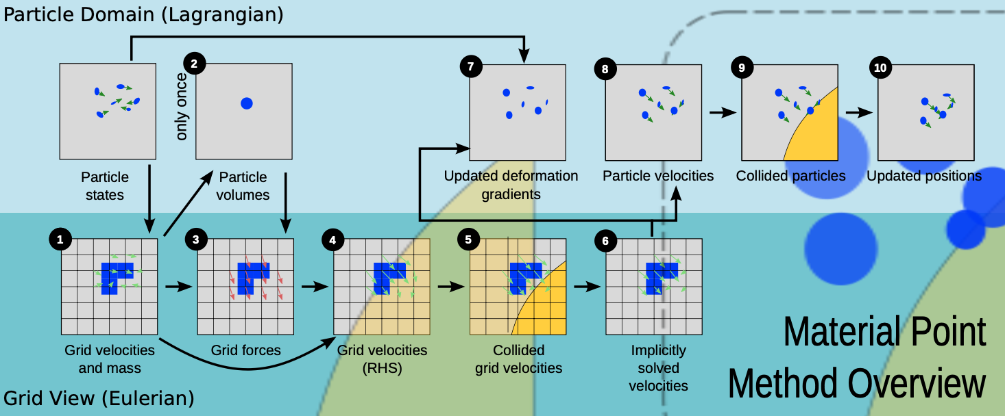
6.1 Overview of MPM
The Material Point Method (MPM) is a hybrid Lagrangian-Eulerian method:
- Lagrangian particles track:
- Mass
- Momentum
- Deformation gradient
- A background Eulerian grid is used to:
- Compute spatial derivatives (e.g., divergence of stress)
- Handle collisions and topological changes (e.g., fracture)
This allows MPM to simulate deformable materials undergoing large strains and discontinuities.
6.2 Deformation Mapping
A body’s deformation is represented as:
\[ \mathbf{x} = \boldsymbol{\phi}(\mathbf{X}) \]
- \(\mathbf{X}\): undeformed (material) coordinate
- \(\mathbf{x}\): deformed (spatial) coordinate
- Deformation gradient:
\[ \mathbf{F} = \frac{\partial \boldsymbol{\phi}}{\partial \mathbf{X}} \]
6.2.1 Governing Equations
Continuum mechanics equations used in MPM:
Conservation of mass: \[ \frac{D\rho}{Dt} = 0 \]
Conservation of momentum: \[ \rho \frac{D\mathbf{v}}{Dt} = \nabla \cdot \boldsymbol{\sigma} + \rho \mathbf{g} \]
Constitutive relation (Cauchy stress): \[ \boldsymbol{\sigma} = \frac{1}{J} \frac{\partial \Psi}{\partial \mathbf{F}_E} \mathbf{F}_E^T \]
Where: - \(\rho\): density
- \(\mathbf{v}\): velocity
- \(\boldsymbol{\sigma}\): Cauchy stress
- \(\mathbf{g}\): gravity
- \(\Psi\): elasto-plastic potential energy density
- \(\mathbf{F}_E\): elastic part of the deformation gradient
- \(J = \det(\mathbf{F})\)
6.2.2 MPM Core Idea
Use particles (material points) to track: - mass $m_p $ - velocity \(\mathbf{v}_p\) - position \(\mathbf{x}_p\) - deformation gradient \(\mathbf{F}_p\)
This Lagrangian approach simplifies mass and momentum updates.
However, since particles have no mesh connectivity, it is hard to compute derivatives like \(\nabla \cdot \boldsymbol{\sigma}\)
6.2.2.1 Eulerian Grid for Derivatives
To handle this: - Use a background Eulerian grid. - Interpolate between particles and grid using basis functions. - Discretize the divergence terms \(\nabla \cdot \boldsymbol{\sigma}\) using Finite Element Method (FEM) in its weak form.
6.2.2.2 Interpolation Weights
They use dyadic products of 1D cubic B-spline basis functions:
\[N^h_i(\mathbf{x}_p) = N\left( \frac{x_p - ih}{h} \right) N\left( \frac{y_p - jh}{h} \right) N\left( \frac{z_p - kh}{h} \right) \]
These weights \(w_{ip} = N^h_i(\mathbf{x}_p)\)are used for: - Transferring data from particles to grid - Interpolating results from grid back to particles
These interpolation functions naturally compute forces at the nodes of the Eulerian grid. Therefore, we must first transfer the mass and momentum from the particles to the grid (P2G).
6.3 MPM algorithm overview
- Rasterize particle data to the grid
- Transfer mass to grid nodes:
\[ m_i^n = \sum_p m_p w_{ip}^n \]
- Transfer velocity to grid using mass-weighted average to ensure momentum conservation:
\[ \mathbf{v}_i^n = \frac{ \sum_p \mathbf{v}_p^n m_p w_{ip}^n }{ m_i^n } \]
⚠️ Note: Unlike FLIP for incompressible fluids, we use normalized weights for velocity.
- Compute particle volumes and densities (first step only)
- Estimate grid cell density: \[ \rho_i^0 = \frac{m_i^0}{h^3} \]
- Weight back to particle: \[ \rho_p^0 = \sum_i \frac{m_i^0}{h^3} w_{ip}^0 \]
- Estimate particle volume: \[ V_p^0 = \frac{m_p}{\rho_p^0} \]
- Compute grid forces
Use the stress-based force formula (Equation 6) with:
\[ \hat{\mathbf{x}}_i = \mathbf{x}_i \]
- Update velocities on the grid
Apply explicit or semi-implicit update (Equation 10):
\[ \mathbf{v}_i^* = \mathbf{v}_i^n + \Delta t \cdot \frac{1}{m_i} \mathbf{f}_i^n \]
- Grid-based body collisions
Handle collisions for \(\mathbf{v}_i^*\) using level sets as described later.
- Solve the linear system
For semi-implicit integration (Equation 9): \[ \sum_j \left( \delta_{ij} + \beta \Delta t^2 \frac{1}{m_i} \frac{\partial^2 \Phi^n}{\partial \hat{x}_i \partial \hat{x}_j} \right) \mathbf{v}_j^{n+1} = \mathbf{v}_i^* \] - Use \(\beta = 1\) for backward Euler. - For explicit updates, just set: \[ \mathbf{v}_i^{n+1} = \mathbf{v}_i^* \]
- Update deformation gradient
Compute new deformation gradient for each particle: \[ \mathbf{F}_p^{n+1} = \left( \mathbf{I} + \Delta t \nabla \mathbf{v}_p^{n+1} \right) \mathbf{F}_p^n \]
Where: \[ \nabla \mathbf{v}_p^{n+1} = \sum_i \mathbf{v}_i^{n+1} \left( \nabla w_{ip}^n \right)^T \]
- Update particle velocities
Use a PIC/FLIP blend (typically \(\alpha = 0.95\)):
\[ \mathbf{v}_p^{n+1} = (1 - \alpha) \mathbf{v}_{\text{PIC}, p}^{n+1} + \alpha \mathbf{v}_{\text{FLIP}, p}^{n+1} \]
- PIC part:
\[ \mathbf{v}_{\text{PIC}, p}^{n+1} = \sum_i \mathbf{v}_i^{n+1} w_{ip}^n \]
- FLIP part:
\[ \mathbf{v}_{\text{FLIP}, p}^{n+1} = \mathbf{v}_p^n + \sum_i (\mathbf{v}_i^{n+1} - \mathbf{v}_i^n) w_{ip}^n \]
- Particle-based collisions
Resolve body collisions again on updated particle velocities \(\mathbf{v}_p^{n+1}\).
- Update particle positions
Move particles forward in time: \[ \mathbf{x}_p^{n+1} = \mathbf{x}_p^n + \Delta t \cdot \mathbf{v}_p^{n+1} \]
6.4 Constituitive model
Simplifications of the constituitive model: - use of principal stretches rather than principal stresses in defining our plastic yield criteria - a simplification of hardening behavior that only requires modification of the Lame parameters in the hyperelastic energy density.
In multiplicative plasticity theory we do:
\[F = F_E F_P\] and we define the model in terms of elasto-plastic energy density:
\[\Psi(F_E, F_P) = \mu (F_p) \|F_E - R_E\|^2_F + \frac{\lambda(F_p)}{2} (J_E - 1)^2\] where - elastic part is given by the fixed corotated energy density - Lame parameters are function of \(F_P\): - \(\mu(F_P) = \mu_ 0 e^{\eta (1-J_P)} \quad \lambda(F_P) = \lambda_0 e^{\eta (1-J_P)}\)
where \(J_X = det(X)\) and \(F_E = R_ES_E\). Here \(\eta\) is the dimensionless plastic hardening parameter.
We define the portion of deformation that is elastic and plastic using the singular values of the deformation gradient. We define a critical compression \(\theta_c\) and stretch \(\theta_s\) as the thresholds to start plastic deformation (or fracture). These two determine when the material starts breaking and the hardening coefficient tells us how fast it breaks.
The deformation as such is elastic for some small deformations around the rest state, dictate by \(F_E\). After it surpasses some critical treshold the plastic regime kicks in. This makes the material stronger under compression (packing) and weaker under stretch (fracture).
6.5 Stress Based forces
Using our defined energy density we can define the total elastic potential energy:
\[\int_{\Omega^0} \Psi(F_E(X),F_P(X))dX.\]
MPM spatial discretization of the stress-based forces is equivalent to differentiation of a discrete approximation of this energy with respect to the Eulerian grid node material positions. That said, we do not actually deform the Eulerian grid so we can think of the change in the grid node locations as being determined by the grid node velocities. If \(x_i\) is the position of grid node \(i\), then \(\hat x_i = x_i +\Delta t v_i\) is the deformed location of that grid node.
Then the MPM approximation to total elastic potential from above can be written as:
\[\Phi(\hat x) = \sum_p V_p^0 \Psi(\hat F_{E_p}(\hat x), F_{P_P}^n)\] where:
\(V^0_p\) is volume occupied by MP in rest state
\(F_{P_p}^n\) is the plastic part of \(F\) at particle \(p\) at time \(t^n\)
\(\hat F_{E_p}(\hat x)\) is the elastic part at \(p\) . We compute it as: \[\hat F_{E_p}(\hat x) = \left(I \sum_i (\hat x_i -x_i)(\nabla w_{ip})^n)^\top\right)F_{E_p}^n\]
\(\hat x\) is the vector of all \(\hat x_i\).
This gives us MPM spatial discretization of the stress-based forces, specifically the force on grid node \(i\) resulting from elastic stresses is:
\[f_i(\hat x) = -\partial_{\hat x_i}\Phi(\hat x) =- \sum_p V_p^0 \partial_{F_E}\Psi(\hat F_{E_p}(\hat x), F_{P_p}^n) (F_{E_p}^n)^\top \nabla w_{ip}^n,\]\[ = - \sum_p V_p^0 \partial_{F_E}\Psi {F_{E_p}^n}^\top \nabla w_{ip}^n.\]
Recall that elastic stress can be related to Cauchy stress so we can write:
\[f_i(\hat x) = -\sum_p V_p^n \sigma_p \nabla w_{ip}^n\] where \(V^n_p = J_p^n V_p^0\) and the stress is:
\[\sigma_p = (J_p^n)^{-1} \partial_{F_E}\Psi (F_{E_p^n})^\top.\] This formulation will help us evolve our grid velocities \(v_i\) implicitly in time.
We can take an implicit step on the elastic part of the update by utilizing the Hessian of the potential with respect to \(\hat x\)
The action of the hessian on some increment \(\delta u\) is:
\[\delta f_i = - \sum_j \frac{\partial^{2}\Phi}{\partial \hat x_i \partial \hat x_j} (\hat x) \delta u_j = - \sum_p V_p^0A_p (F_{E_p}^n)^\top \nabla w_{ip}^n\] where
\[A_p = \frac{\partial^2 \Psi}{\partial F_E \partial F_E}(F_E(\hat x), F_{P_p}^n) : \left(\sum_j \delta u_j (\nabla w_{jp^n}^\top F_{E_p}^n\right).\]
6.6 Semi-Implicit Update
We define the updated grid node positions as: \[ \hat{\mathbf{x}}_i = \mathbf{x}_i + \Delta t\, \mathbf{v}_i \] Since we never actually deform the grid, we consider \(\hat{\mathbf{x}}\) as a function of the grid velocity \(\mathbf{v}\), i.e. \(\hat x(v)\).
Let: - \(\mathbf{f}_i^n = \mathbf{f}_i(\hat{\mathbf{x}}(0))\) - \(\mathbf{f}_i^{n+1} = \mathbf{f}_i(\hat{\mathbf{x}}(\mathbf{v}^{n+1}))\)
which gives us \(\frac{\partial^2 \Phi^n}{\partial \hat x_i \partial \hat x_j} = - \partial_{\hat x_j}f_i^n\)
We approximate the time evolution of velocity with a semi-implicit integration scheme: \[ \mathbf{v}_i^{n+1} = \mathbf{v}_i^n + \Delta t\, m_i^{-1} \left[ (1 - \beta)\mathbf{f}_i^n + \beta\mathbf{f}_i^{n+1} \right] \] Now use a Taylor expansiom for \(\mathbf{f}_i^{n+1}\):
\[ \mathbf{f}_i^{n+1} \approx \mathbf{f}_i^n + \sum_j \frac{\partial \mathbf{f}_i^n}{\partial \hat{\mathbf{x}}_j} \Delta t\, \mathbf{v}_j^{n+1} \] Substituting this approximation gives the update for grid velocities: \[ \mathbf{v}_i^{n+1} \approx \mathbf{v}_i^n + \Delta t\, m_i^{-1} \left( \mathbf{f}_i^n + \beta \Delta t \sum_j \frac{\partial \mathbf{f}_i^n}{\partial \hat{\mathbf{x}}_j} \mathbf{v}_j^{n+1} \right) \]
6.6.1 Linear System
To solve for \(\mathbf{v}^{n+1}\), we rearrange terms into a linear system: \[ \sum_j \left( \delta_{ij} \mathbf{I} + \beta \Delta t^2 m_i^{-1} \frac{\partial^2 \Phi^n}{\partial \hat{\mathbf{x}}_i \partial \hat{\mathbf{x}}_j} \right) \mathbf{v}_j^{n+1} = \mathbf{v}_i^\star \] where: \[ \mathbf{v}_i^\star = \mathbf{v}_i^n + \Delta t\, m_i^{-1} \mathbf{f}_i^n \] - Matrix is symmetric and positive definite - Solved efficiently with Conjugate Residual method - Requires ~10–30 iterations per time step
6.6.2 Deformation Gradient Update
Step 1: Predict Elastic Deformation
We compute an initial trial elastic gradient from the velocity gradient: \[ \hat{F}_{E_p}^{n+1} = \left( \mathbf{I} + \Delta t\, \nabla \mathbf{v}_p^{n+1} \right) F_{E_p}^n \] Set: \[ \hat{F}_{P_p}^{n+1} = F_{P_p}^n \] So: \[ F_p^{n+1} = \hat{F}_{E_p}^{n+1} \hat{F}_{P_p}^{n+1} \] Step 2: Clamp Excess Deformation Now we take the part of the elastic \(F\) that exceeds the critical deformation threshold and push it into plastic \(F\). We perform SVD on the trial elastic part: \[ \hat{F}_{E_p}^{n+1} = U_p \hat{\Sigma}_p V_p^T \] Clamp singular values to the allowed range: \[ \Sigma_p = \text{clamp}(\hat{\Sigma}_p, [1 - \theta_c, 1 + \theta_s]) \] Step 3: Redistribute Deformation
We update the elastic and plastic parts as:
\[ F_{E_p}^{n+1} = U_p \Sigma_p V_p^T \]
\[ F_{P_p}^{n+1} = V_p \Sigma_p^{-1} U_p^T F_p^{n+1} \]
So the decomposition satisfies:
\[ F_p^{n+1} = F_{E_p}^{n+1} F_{P_p}^{n+1} \]
- Excess deformation (beyond yield) is moved from elastic to plastic part
- Guarantees energy is dissipated through plastic flow
- Keeps elastic stress in a physically valid range